The Mathematics of Build Queue Optimization and Auto-Scaling

Archival Note: This is an archived version of a three-part blog post series originally published on the CircleCI blog in the spring of 2016 by Kevin Bell (GitHub: bellkev) — Part 1 on March 28, 2016, Part 2 on April 6, 2016, and Part 3 on April 18, 2016. The original posts have since been removed from CircleCI’s website (this copy is reconstructed from the Internet Archive, including the original figures). I’ve lightly edited the content to be less CircleCI-specific while preserving the technical insights and mathematical analysis. The original simulation code is still available at bellkev/asg-sim.

These posts remain one of the clearest explanations of applying queueing theory to CI/CD infrastructure that I’ve encountered, and the conclusions are applicable to any continuous integration system.

Part 1: Why Build Queues Are Costly

Over the past several years, continuous integration services have run millions of builds on rapidly growing fleets of build containers. Operators have tweaked and tuned countless parameters to ensure their auto-scaling clusters of servers always have capacity to run builds while minimizing unused resources.

A New Challenge

After the launch of on-premises CI solutions, many teams started asking: how should we run our own builds in AWS Auto Scaling groups or similar services? Does auto scaling make sense for them? What parameters will keep their CI instance responsive while minimizing idle server time?

The problem is that these teams don’t want a several-thousand-container cluster to process thousands of builds per hour from a globally distributed pool of developers. They want a few hundred containers to process dozens of builds per hour from a couple buildings’ worth of developers. They also use different machine types, different container specs, and have different traffic patterns from large SaaS CI providers.

We need to understand not just how to run one giant-sized cluster, but how to optimize dozens of heterogeneous, medium-sized clusters.

Thinking about this problem, it occurred to me that there might be a way to model it with a bit of queueing theory. The simple case of a single server running jobs of a fixed duration occurring randomly in time (following a Poisson distribution) is known as an M/D/1 queue, and there are simple closed-form solutions to the expected wait time in such a queue. The multi-server (M/D/c) case has much more complicated closed-form solutions, but adding auto scaling quickly makes the problem intractable. Or at least I didn’t find an answer after several minutes of spirited googling, which is practically the same.

An Experimental Approach

This is where I could’ve built some kind of elaborate computational simulation of auto scaling build clusters and run millions of iterations of Monte Carlo experiments with hundreds of thousands of possible parameters, so of course that’s what I did. It lives at bellkev/asg-sim, and I’ll be using data from that model in the rest of this post.

I should also highlight that while I’m focusing on modeling build clusters, much of what I cover will also apply to selecting appropriate infrastructure sizing or managing clusters of servers running arbitrary jobs.

Before tackling auto scaling, I spent time on the fixed-fleet-size case, because that is the basis of comparison for all auto scaling solutions. After verifying that my model matched the theoretical predictions for the simple M/D/1 case, I started on the problem of balancing queue time and resource utilization.

It’s obviously easy to do a good job of just one of these things. You can underprovision and keep your queue full and machines busy, or you can overprovision and keep your queue empty and your machines idle. The following graph makes this clear.

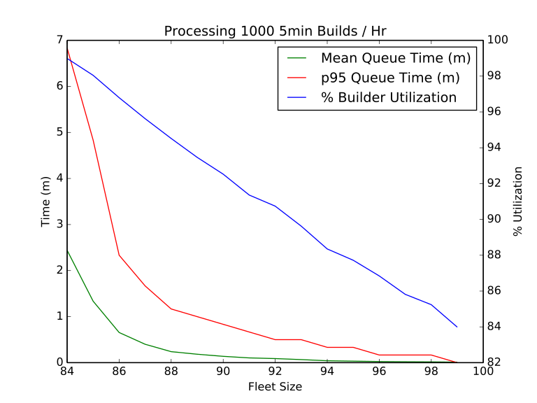
This graph shows what happens when the same traffic pattern is run against fixed-size clusters of varying sizes. Clearly smaller clusters have higher machine utilization with long queue times and larger clusters have low utilization with short queue times.

A Cost Function

In order to choose some kind of balance point, we need to do a bit of hand-wavy math. Developers’ time is valuable, so there should be some kind of dollar value that can be placed on time they spend waiting for builds in the queue. Large servers are also expensive, and there is a cost associated with keeping them running. You can model the total cost something like this:

cost = idle machine hours × cost per machine hour +
       queued build hours × cost per developer hour

You may be philosophically opposed to the idea of equating human hours to machine hours, or you might argue that five minutes waiting on a build really causes more like thirty minutes of lost productivity because of the interruption it causes. You might even think that queueing time doesn’t really matter, because developers can go get coffee or work on some other feature while their builds run.

I would argue that this is absurd, because if developers have to take an arbitrarily long break or context switch after each push to CI, then what kind of unmeasurably bad outcomes are you incentivizing?

We only need to get the cost parameters accurate to within a factor of ten or so, so don’t worry about it too much. I’ll be using $200 (maybe a little high, but interruptions are expensive) per hour of developer time and AWS m4.large on-demand rates for machine hours unless otherwise stated.

A final point worth making before we proceed is that slow builds are still exactly as bad no matter what. Using the parameters above, the cost of actually running a build looks like this:

build running cost = build run time ×
                     (cost per machine hour + cost per developer hour)

Obviously this is terrible, because it takes both compute resources and developer time, but this number only depends on the build run time, number of builds, and other cost parameters. You should absolutely work hard to minimize this cost, but it’s a separate problem from optimizing away the waste cost of under/overprovisioning your build cluster.

Running the Numbers

Okay, now that we’ve defined a reasonable cost function for our model, we can look at the fleet size experiment from before in terms of a cost curve. (The dollar amounts are basically arbitrary. They’re big because I ran the simulation for the equivalent of months with hundreds of servers for each data point to make the graph nice and smooth.)

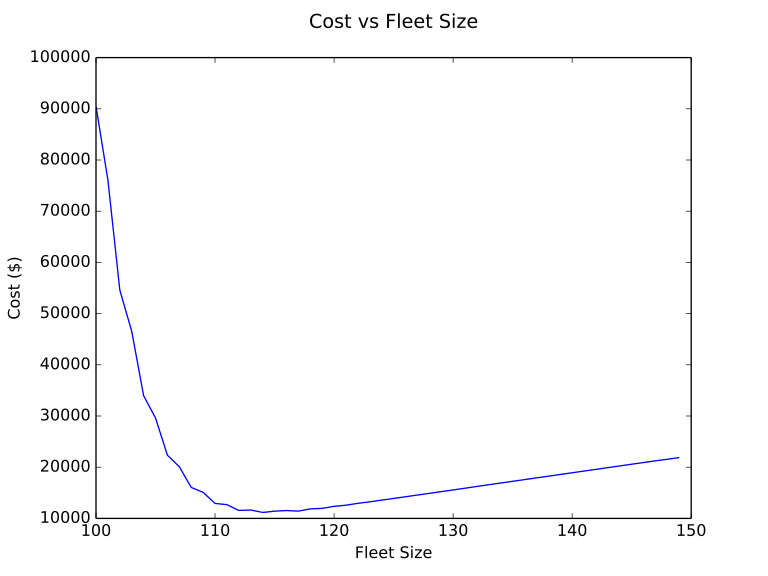
The curve is obviously not symmetric, but that makes sense if you think about it. In queueing theory, a queue that gets added to faster than it can process jobs is considered “unstable” and quickly grows to infinity. Even stable queues will occasionally grow a bit due to random spikes in traffic, leading to some average queue length, but that average queue length blows up asymptotically as the system approaches the unstable limit. On the other side of the curve, there is a simple linear growth in cost as we add builder machines to the fleet.

If we produce one of these curves for various traffic patterns, we can come up with optimum fleet sizes for those workloads by taking the minima. Here’s what we get for 5-minute builds getting triggered at various frequencies.

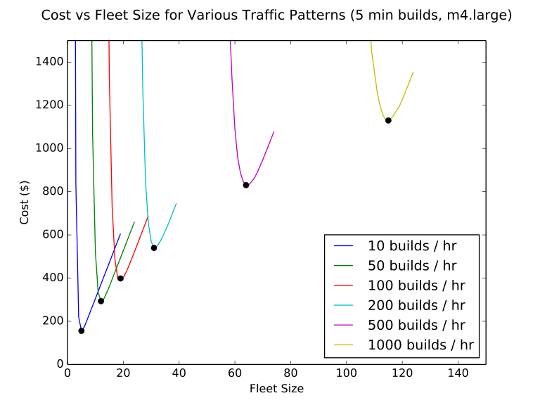
Now that we have optimum fleet sizes in terms of cost, let’s see what queue times and levels of machine utilization are considered optimum for a fixed-size fleet.

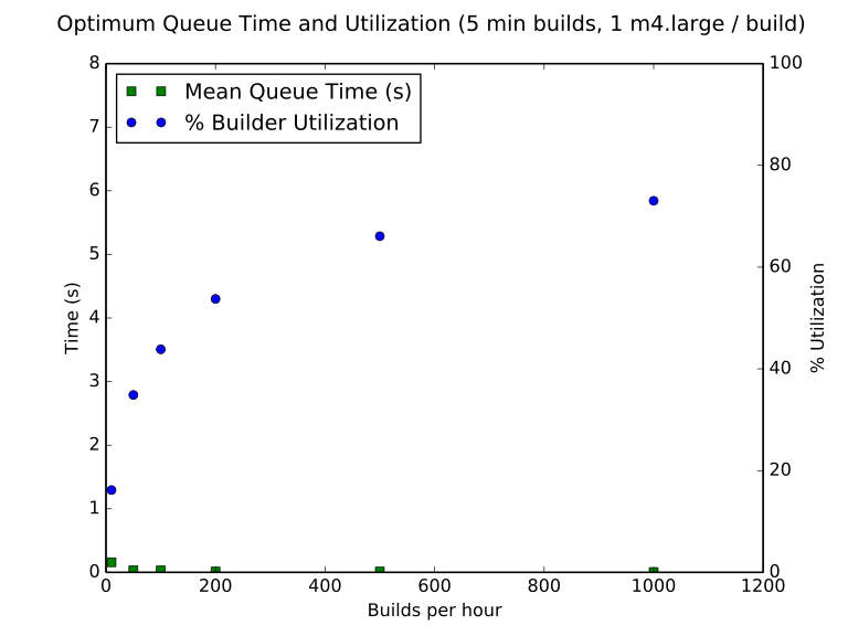
Look at that! The queue times are virtually zero, even if it requires keeping machines at under 20% utilization for smaller fleet sizes. Remember, this is even in the model where we treat developers as simple, swappable, fixed-price cogs in the machine. It still clearly pays off to keep queue times low. Also notice that you get some economy of scale as the traffic and fleet size grow.

The picture is similar if we look at varying build times at fixed number of builds per hour.

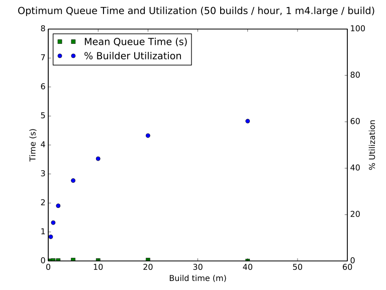
Only this time we get increased utilization for slower builds. This is a bit of a silver lining around the dark cloud of slow builds, but obviously not something to strive for.

Is This For Real?

There are certainly valid possible objections to the conclusion so far. For example, what about a team that runs builds on expensive hardware, lives in an economy where developers are a bit cheaper, and doesn’t consider waiting on builds to be “that bad”?

Even if my assumptions are orders of magnitude off, each build requires the equivalent of two m4.10xlarge machines at on-demand prices, and developers earn starvation wages, the result is nearly the same:

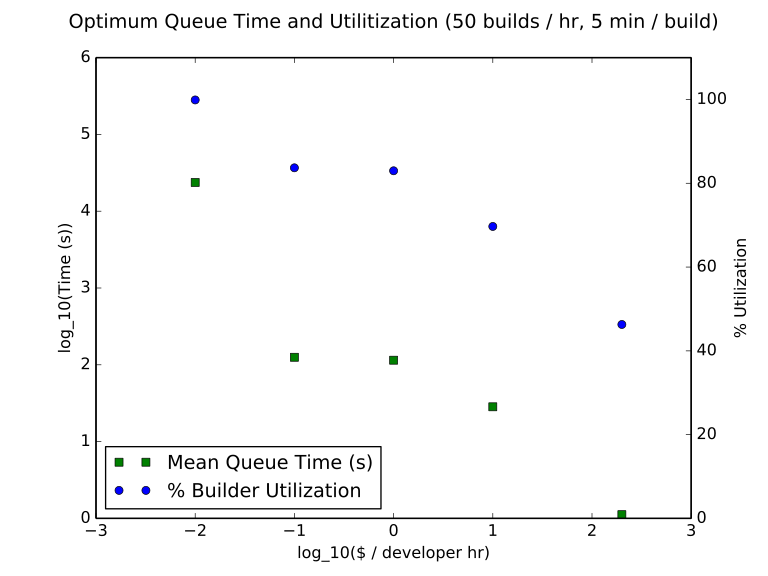
Even with super expensive hardware, letting builds queue for more than 10 seconds isn’t cost effective unless developers make about ten dollars per hour. Letting builds queue for more than a minute is equivalent to valuing your developers’ time at less than a dollar per hour, and letting builds queue for more than ten minutes only makes sense if developers make pennies per hour.

“Letting builds queue for more than a minute is like valuing your developers’ time at less than a dollar per hour.”

My theory as to why such queueing is still commonplace is that most organizations don’t look at the cost of their build infrastructure side-by-side with the cost of their developers. Instead, build machines are likely an expense that some team lead is incentivized to reduce, while salaries are more opaque and decided at a higher level. The productivity loss due to queuing builds is hard to measure or quantify, so it gets swept under the rug as one more excuse of lazy, complaining developers.

Conclusion (Part 1)

Fortunately the results of the experiment so far can be distilled down to some very simple advice. If you need to decide how big to make your fixed-size build cluster, set it at whatever size leads to zero queueing. When I say zero, that means less than a second on average for most workloads and under about 10 seconds on average even if you run your builds on expensive hardware.

You will enjoy greater machine utilization as traffic (or build run time) increases, but you shouldn’t worry about that. Always target near-zero queue time.

I should also highlight that this simulation does assume that the timing between builds is random, and not influenced by the queue time itself. In a team with chronically queuing builds, it’s probably common for developers to avoid pushing or skip CI when the queue is long. But again, is that behavior that you want happening in your team? Probably not!

Hold on though, what about auto scaling? Isn’t it supposed to save the day and let us achieve web scale? Well, let’s find out…

Part 2: The Challenge of Auto-Scaling Against Random Traffic

In Part 1, I introduced a computational simulation of build clusters and used it to determine optimal build fleet sizes taking both machine costs and developer waiting costs into account. The ultimate goal is to learn how best to manage an auto scaling build fleet, but I started with the case of a fixed-size fleet to get a baseline to improve on. Now the auto scaling begins!

Reviewing Fixed-Size Fleets

The cost of developers waiting for queued builds caused the cost model to always prefer near-zero queueing. This was accomplished by making the build fleets large enough to absorb any spikes in traffic, sometimes by a surprising amount.

For example, five-minute builds triggered at an average rate of fifty per hour, or an average load of 250 build-minutes per hour, could ideally be handled by less than five machines if the builds were timed perfectly. The model recommended twelve machines for this traffic pattern though. Here is a plot of the simulated usage of such a cluster:

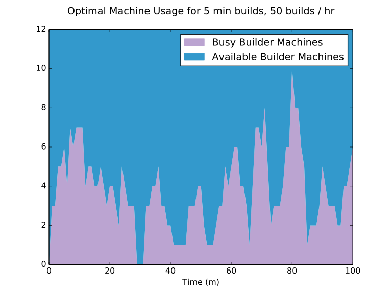
The queueing associated with these spikes “breaking through” would quickly undo the savings that could be gleaned from a smaller fleet by wasting expensive developer time. The twelve-machine fleet is needed to handle the random spikes in traffic, but this results in a lot of machines sitting idle.

Let’s Auto Scale!

Hopefully instead of just leaving all this extra capacity lying around in case a spike in usage happens, we can use auto scaling to resize our fleet dynamically. The way auto scaling works (at least as implemented with AWS Auto Scaling groups and CloudWatch Alarms) is that there is some metric that you want to hold within some acceptable range—in this case we’ll use the number of available builder machines—and whenever the metric strays outside of that range, the auto scaling mechanism responds by adding or removing machines to the fleet as needed.

While the promise of a continually resized fleet is exciting, it introduces a lot more parameters to adjust compared to a fixed-size fleet. Instead of just a number of machines, we can now vary the thresholds (high and low) that trigger scaling, the frequency with which the metric is sampled (the CloudWatch Alarm period in AWS), the number of periods in a row the metric needs to be past the threshold for scaling to happen, and how many machines to add or remove at once.

The volume of builds and their durations will continue to influence the performance of the cluster, but now we also need to think about the time it takes to add builder machines to the fleet—basically the boot time—as this determines the time lag associated with accommodating sudden changes in traffic.

To the Cloud!

All of these new settings result in a huge, many-dimensional parameter space over which we need to minimize our cost model. I started to map out the space with a handful of traffic patterns that I modeled with fixed-size fleets and used them as upper bounds for scaling thresholds (because they already did a good job of keeping queues near zero), then I varied boot times and the rest of the auto scaling parameters over reasonable ranges.

This resulted in a few hundred thousand combinations of settings and several thousand years of simulation time to run. After some cursory profiling and performance enhancements, this turned out to be about a 12-hour job for my laptop.

This is where I could have spent a lot of valuable time looking for some fancy data science to streamline the search, but instead I decided to follow my own advice from the last section regarding the cost of human time vs. computer time and delegated to several dollars-worth of c4.8xlarges. I just had to write a bit of code to serialize the inputs and outputs to my model into hunks of JSON that were readily rsyncable with EC2 machines, and I was off to the races.

The Data

After analyzing reams of cloud-enabled data, the prospect of saving much money on a build cluster with realistic parameters was grim. Let’s first look at one of the more predictable results. If you want to be able to auto scale based on quickly changing metrics, fast boot times are key.

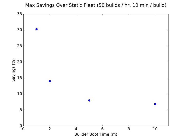
The savings we get from auto scaling plummets as the boot time of builder machines increases. If you look back at the spikey build traffic graph at the top of this section, this should make sense. If we launch machines in response to a spike in traffic, and they aren’t ready until after the spike has passed, then they won’t do any good.

Next let’s look at the best auto scaling outcomes relative to the length of each build.

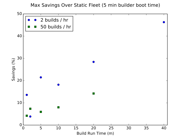
Sadly we only get compelling savings for very slow, infrequent builds. Keep in mind that this model is idealized in a lot of ways, so predicted savings of 10-15% are likely not to materialize in the real world.

We can look at the same general picture by looking at savings vs. build frequency while holding build length constant.

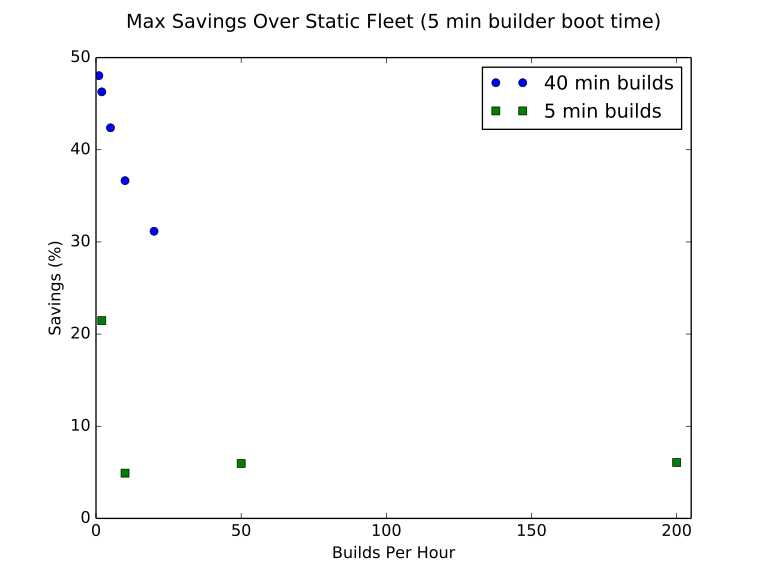
Again, we only see compelling savings for slow, infrequent builds. Looking at the fleet capacity and usage over time can help us understand why autoscaling only seems to help for this scenario with slow, infrequent builds.

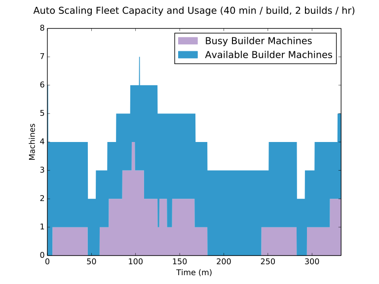
The builds are slow enough that the fleet is able to scale up to handle new traffic over the course of a single build, and builds are infrequent enough that it’s unlikely for a bunch of builds to be kicked off in the middle of scaling.

The Timing Just Isn’t Right…

Unfortunately for our auto scaling project, most organizations don’t trigger only two builds per hour, with builds that last forty minutes each. In fact either of those numbers is probably indicative of an unhealthy software team.

An organization running their own CI infrastructure is more likely to have dozens or hundreds of builds per hour, meaning an average of one or two minutes between builds at most. Each build should also take only a few minutes at most.

The fundamental problem is that boot times on the order of minutes are just too slow to scale in response to the minute-to-minute random traffic fluctuations of most build fleets. Even a boot time of one minute would be too slow under heavier traffic, especially when combined with the added delays of the AWS CloudWatch periods and Auto Scaling groups.

The… End?

If we were talking about a cluster of containers that could boot in seconds instead of VMs that boot in minutes, that would change things dramatically. That could be a game changer in the coming years, but at the moment most organizations don’t have such a container cluster.

There is also the issue that to be able to scale, a container cluster would have to have some idle or low-priority capacity to scale “into”. A pool of containers running offline ETL jobs or other pausable work would be a great candidate to kill off in favor of builds (the canonical example from Google is search indexing jobs), but again, most organizations aren’t there yet.

There is another critical factor that I’ve ignored so far that the astute reader is probably already thinking about. Everything in the model so far has made the major simplification that the timing between builds is random but occurs at some constant average rate.

Of course this doesn’t actually describe real build clusters, because real programmers don’t push code at 4am, or at lunch time, or on New Year’s Day (unless they’re total 1337 10Xer ninjas). These kinds of hourly or daily traffic fluctuations are much more manageable with auto scaling even if booting builder machines takes two, five, or even ten minutes, and we’ll learn all about it next…

Part 3: When Auto-Scaling Actually Works

So far in this series, I’ve introduced a computational model of auto scaling build fleets and used it to try auto scaling against randomly varying loads of builds. We hit a bit of a snag in Part 2 when we realized that VM boot times were just too slow to allow scaling in response to random fluctuations in real-world traffic. This time, we’re going to take into account fluctuations in traffic throughout the day and see if auto scaling can help us there.

Fire Up the Data Analysis

Let’s look at how often actual development teams build throughout the day. Looking at any given day for a single company would be pretty random and spikey-looking, but totaling up all the builds in given time windows over a number of days yields some nice smooth curves. Remember, these curves would be flat lines if builds happened randomly at a constant rate throughout the day, but clearly that’s not the case.

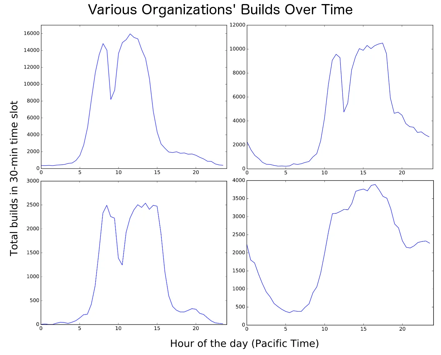
The plots of builds run over time mostly look like mittens, with a little dip at lunch time. Except for Organization 4, which seems to either not eat lunch or perhaps be more globally distributed.

If you add up all the builds across many organizations, you get a plot that looks like this:

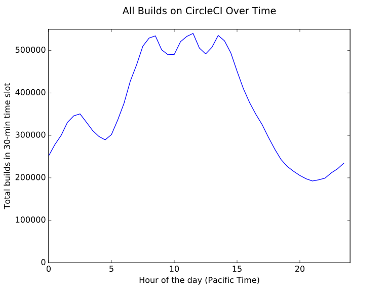
It’s sort of a sine wave with a couple of lunch times and a few employees located in Europe. It’s reasonable to assume that a very large company with teams all around the world sharing a central build cluster would start to look something like this.

Stationary Arrival Patterns Are So Out

To model this time-varying traffic, we’re just going to make one change to the simulation. We’ll keep all the random spikeyness from before, because the auto scaling process still definitely needs to handle it, but we’ll add a time-varying function to multiply our random distribution by before sampling it.

To keep things simple, I’m going to use a sine function that varies from 0 at midnight, up to 1 at noon, and back down to 0 at midnight. I’ll multiply the same traffic patterns from before by this function, so what used to be the constant traffic rates will now be the peak traffic rates.

The Big Reveal

The nuts and bolts of testing this new traffic pattern are basically identical to last time, with one quick blast of c4.8xlarge action to run through all the possible autoscaling parameters. Before analyzing the results further, I’ll share a quick sample of what an arbitrary day’s worth of simulation time looks like under this traffic pattern:

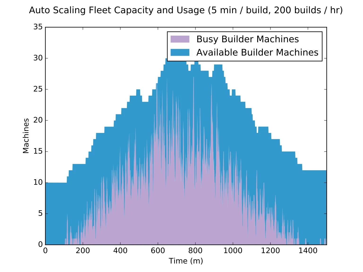
Yeah! Now that’s what I call auto scaling! Notice how violent the spikes can be, and that the model is optimized to just barely absorb them. Also notice the big, solid chunk of high utilization in the middle of the day that represents constant utilization of a good chunk of the fleet, which is good for machine efficiency.

After looking at that graph, this plot of savings over fixed-size fleets with the new traffic pattern shouldn’t be surprising:

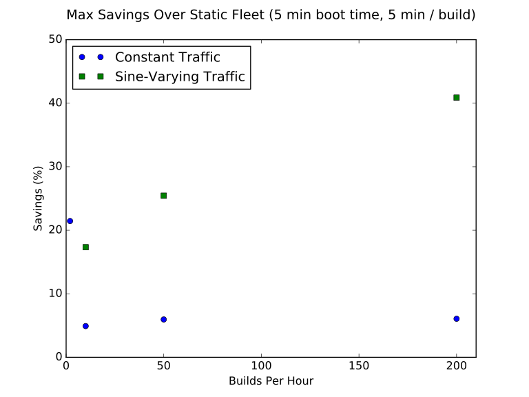
First, we save a lot more for each traffic level compared to the constant-traffic case. Second, and more importantly, the savings don’t decrease but increase with traffic. When we tried to auto scale against random traffic spikes, more traffic just meant more randomness and spikeyness. When scaling against a more slowly moving base traffic rate though, more traffic means we have a solid foundation of usage (the big purple hunk in the graph above), while still being able to shut off most of the machines at night.

So How Do I Set Up Auto-Scaling Already?

My primary goal when I started this exercise was to determine if auto scaling made sense for real-world boot times and traffic patterns, and if so, what auto scaling parameters yield the best performance?

The answer to the first part of the question seems pretty clear based on the results covered in this post and the previous one. Auto scaling against random, minute-to-minute fluctuations in build traffic doesn’t make sense for realistic boot times and traffic patterns, but scaling according to hour-to-hour changes in traffic definitely does.

The second part of the question, about what parameters are best for any given traffic pattern, is much more difficult. My brute-force approach was useful to determine that parameters do exist for which auto scaling saves a lot of money for daily traffic patterns, but that’s not enough to be able to prescribe a complete set of e.g. AWS Auto Scaling group (ASG) parameters for any case. That’s a complicated, many-dimensional modeling problem even in my idealized model, with more complexity in the real world.

That said, I did a bit of simple analysis of the parameters turned up by my optimization effort and found a few clear trends. I captured these in a simple formula to recommend ASG parameters (CloudWatch Alarm timings, thresholds, etc) for a given load. The formula depends only on the overall volume of builds (build minutes per hour) and not on the length of builds, so hopefully it works around the simplification that build times are constant in my model. The formula appears to do a reasonably good job in recommending parameters even for traffic that was well outside of the search space of my brute-force approach:

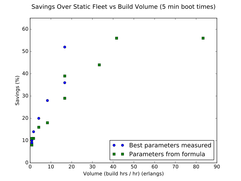
Note that the formula only does so-so relative to the optimum parameters found by my brute-force search in the area it covered, which is expected because I didn’t capture every possible predictor of good performance in my formula. However, the formula goes on to perform very well in higher-volume cases, which is again expected because those cases should have a bigger foundation of running builds to scale around. It would probably be silly to do much more than this rough pass at recommended parameters based on my model without gathering more real-world data from production clusters.

Key Takeaways

After this extensive exploration of queueing theory and auto-scaling for CI/CD build fleets, here are the key insights:

1. Always Target Near-Zero Queue Times

The mathematics are clear: even with conservative cost assumptions, letting builds queue for more than a few seconds is equivalent to valuing your developers’ time at poverty wages. The productivity loss from context-switching and waiting far outweighs the cost of additional compute capacity.

2. Auto-Scaling Against Random Spikes Doesn’t Work

With realistic VM boot times (1-10 minutes), auto-scaling cannot respond quickly enough to handle the minute-to-minute random traffic fluctuations typical of healthy CI/CD workloads. You’ll need enough baseline capacity to handle these spikes anyway.

3. Auto-Scaling Against Daily Patterns Works Great

Auto-scaling does provide significant cost savings when scaling against predictable daily traffic patterns (business hours vs. nights/weekends). This works because the time scales involved (hours) are much longer than VM boot times (minutes).

4. The Simulation Approach Generalizes

While this analysis focused on CI/CD build infrastructure, the same principles and modeling approaches apply to any job-processing cluster where:

• Jobs arrive at varying rates
• Developer or user wait time has a cost
• Infrastructure has both fixed and variable costs
• Traffic patterns are somewhat predictable

5. Context Switching Is the Hidden Cost

The reason queue times are so expensive isn’t just the waiting—it’s the context switching and interruption to flow state. A developer waiting for a 10-minute build doesn’t lose 10 minutes; they lose potentially an hour of productivity.

Further Exploration

The original simulation code is available at bellkev/asg-sim for anyone interested in:

• Testing more traffic patterns and parameters
• Exploring alternative auto-scaling metrics and models
• Adapting the model for their own infrastructure challenges
• Understanding the implementation details of the queueing simulations

I encourage any operators of build clusters, job processing systems, or anyone curious about applying queueing theory to infrastructure problems to take a look!